Order Quantity Control in Excel – Part 3

The article participated in the 3rd edition of the “Piórem Logistyka” competition.

During this stage, it is important to determine the type of distribution for the studied characteristic. With this information, it will be possible to estimate the parameters of the theoretical distribution, approximated by the empirical cumulative distribution function. In the developed model, the identification of the distribution type was performed using tabulation (Figs. 6, 7). As a result of measuring the values of specific system characteristics (demand size and order lead time), a sequence of values described in column 2 is obtained (Figs. 6 and 7).

Observations can be divided into:

disjoint classes of the same length equal to:

where: denote, respectively: class length, number of classes, the n-th value of the sequence ordered in ascending order, the first value of the sequence.

Consequently, the r-th class ( r= ) includes those observations that satisfy the inequality:

<

The class midpoint can be determined from the formula:

After determining the number of classes, the number of elements in a class, and the class midpoints, one should use the classical definition to establish class probabilities. Pairs: class midpoint and the probability of elements belonging to classes form a probability distribution, which can be written in the form of a table.

To generate pseudorandom numbers with an identified distribution (Figs. 5, 8), the predefined spreadsheet function f(x)=Rand()³ (Fig. 4) was used. It generates numbers from the interval (0,1) according to a uniform distribution.

The generated auxiliary number is identified with the corresponding class number (Figs. 6, 7). The midpoint of the obtained class can be the generated number x with the distribution shown in the chart (Figs. 5, 8). The model (Fig. 4) retrieves values from two distribution tables (Figs. 6, 7): demand and order lead time, along with their probabilities. Their values are generated in the model using the above technique.

Fig. 5. Probability distribution by classes for demand (own elaboration based on: A. Manikowski, Z. Tarapata, Forecasting and simulation of enterprise development, WSE, Warsaw 2002)

Fig. 6. Tabulated probability distribution for demand (own elaboration based on: A. Manikowski, Z. Tarapata, op. cit.)

Fig. 7. Tabulated probability distribution for order lead time (own elaboration based on: A. Manikowski, Z. Tarapata, op. cit.)

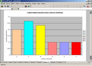
Fig. 8. Probability distribution by classes for order lead time (own elaboration based on: A. Manikowski, Z. Tarapata, op. cit.)

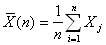
The results of a single simulation can be treated as a statistical sample. However, it must be remembered that as a result of conducting a second experiment with a different set of independent pseudorandom numbers, the estimates will be different. This is due to the presence of random elements in the model. A proper evaluation of the model consists of analyzing the results of many experiments and applying several standard procedures. One should estimate the parameter x of the system’s functioning (total daily inventory cost) based on the results from n experiments (simulation runs). The estimate of the expected value of parameter x is the arithmetic mean of the obtained results:

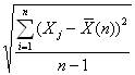
The standard deviation of the arithmetic mean of n independent random variables is calculated from the formula:

=

We run the simulation using the dialog box shown in Fig. 9.

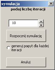
Fig 9. Dialog box for simulation (own elaboration)