









Risk assessment in the logistics transport process – part 1
Obtaining a new operating model and a specific form of the Hasse diagram has consequences for the costs of implementing the logistics transport process. As a result of the operation performed, a splitting of propositional variables occurs.
These variables reflect the risk factors occurring in the examined transport process, characterized by a specific probability and consequence of the occurrence of risk factors, meaning that the duplication of activities will translate into the final level of costs. By applying the principle of characterization, it is easy to see that the occurrence of risk factors has consequences not only at the place where the event occurs. The effects often translate into other areas of the company’s operation, and even into the entire organization. After the characterization is completed, we can calculate the actual costs of the occurrence of risk factors.
Obtaining information about the actual costs incurred by the company in connection with the occurrence of risk factors, showing the structural-functional dependencies of the model, was described using the example of research conducted in Company K. The AWZR simulator will be used to conduct the analysis.
Example
Based on data obtained during research conducted in 2008 in Company K, a propositional function describing the occurrence of risk factors in the logistics transport process was determined. The propositional function is obtained by selecting the first module propositional function model (Figure 1). We enter a list of risk factors occurring in the company and information about the probability and consequences of their occurrence.
To obtain the propositional function, we select the Company, a specific year, and mark in the “selection” column those risk factors whose analysis we want to perform (cf. Figure 1).
9 out of 24 risk factors listed in Table 1 will be subjected to analysis. On this basis, the propositional function took the following form:

The operating model Ψa of the propositional function ZPx is given as a compilation:
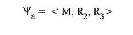
where:
M – set of propositional variables;
R2 – set of relations defined by 2-element alternative terms describing the production, distribution area,
R3 – set of relations defined by 3-element alternative terms describing the supply, transport, warehousing, logistics process management area)
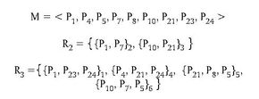
The simulator operating model module of AWZR allows for obtaining a graphical form of the operating model (Figure 2). The graphical form is created as follows: for each propositional variable occurring in the operating model, the number of the conjunction in which it occurs is determined: P1 (1,2), P4 (4), P30 (3,6), P21 (3,4,5), P23 (1), P7 (2,6), P8 (5), P5 (5,6), P24 (1,4). Propositional variables constitute the vertices of the graph. Variables occurring in the same conjunctions are connected by lines. Thus, in Figure 2, propositional variables occurring in the first conjunction are connected by a red line, in the second by a green line, in the third by a blue line, in the fourth by a black line, in the fifth by a yellow line, and in the sixth by a purple line.
The article comes from the magazine “Logistyka” 2/2012.